

Chart types
Set up a pivot table
Cross-tab measures by row and column groups, and set the columns in Pivot Settings.
Group measures by rows and columns in one table.
Before you start
- The metric is grouped: it has at least one dimension and a measure with an aggregate. Pivot Table does not show until then.
Steps
-
Add the group fields to Dimensions, for example
regionandmonth. -
Add the values to Measures, for example
sum(revenue). -
In the chart toolbar, select Chart type, then Pivot Table.
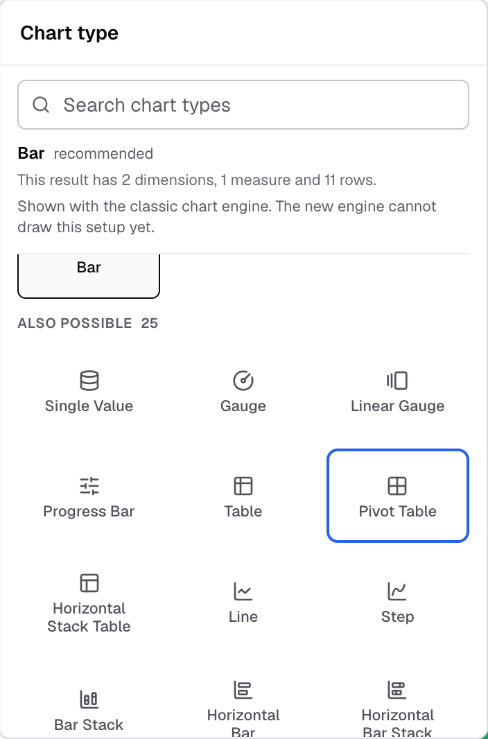
Pivot Table in the Chart type picker. -
In the chart toolbar, select Pivot. The Pivot Settings panel opens at the side.
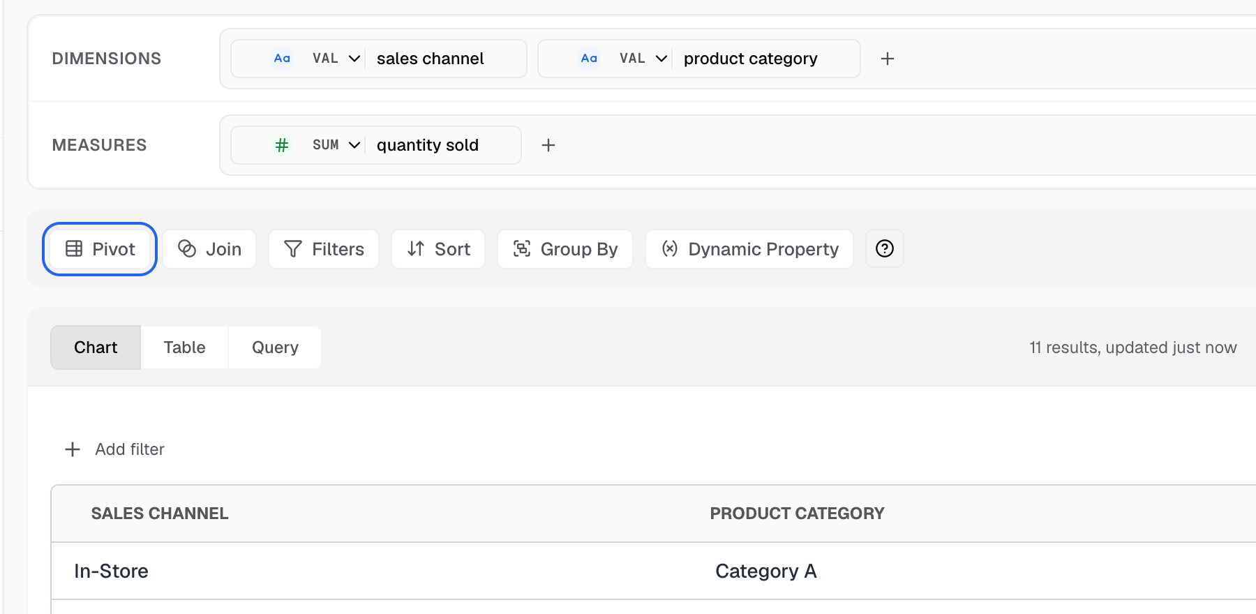
Pivot is the first button in the Query toolbar for a pivot table. -
In Columns, choose the dimensions to group by. Check the preview after each change.
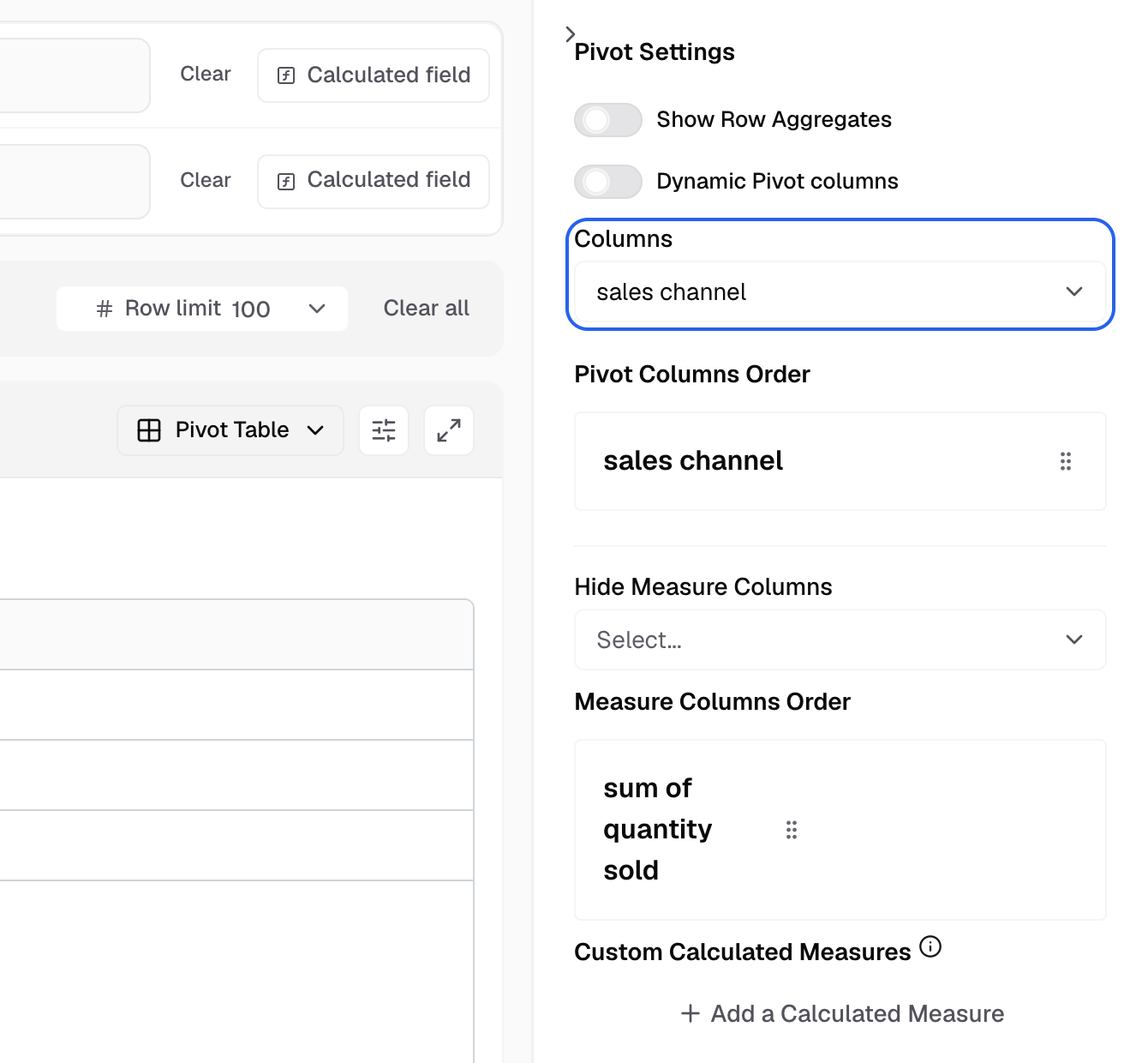
Columns sets the dimensions that become column headers. -
Set the other options you need. See Pivot settings.
-
Save the metric.
Pivot settings
| Setting | What it does |
|---|---|
| Show Row Aggregates | Adds a total for each row group. |
| Dynamic Pivot columns | The columns follow the values in the data. |
| Columns | The dimensions the table groups by. |
| Hide Measure Columns | Hides the measures you pick from the table. |
| Measure Columns Order | Sets the order of the measure columns. |
Settings for this chart
Select Appearance in the chart toolbar. A pivot table has two tabs, Appearance and Actions. On Appearance:
- Number format
- UI styling: header, text wrap, content font, dividers and borders.
- Conditional formatting
- Formatting
Drill down and Chart Click Actions do not work on a pivot table.
Next: change how the chart looks.